In data science, standing out can be both a strength and a challenge. Data anomalies are samples in a dataset that deviate from the expected “normal behavior”. While they can represent wrong data that shouldn’t have been included in the first place, they can also uncover rare and underrepresented scenarios, essential for improving data quality and ensuring robust and safe AI decision-making.

In this article, we will showcase audio anomalies in the SpeechCommands dataset and highlight:
- Anomalies at different levels of granularity including acoustic and quality-based anomalies such as low-pitch, mumbling, and truncated commands.
- How anomalies can be found, visualized, and curated at scale.
- How anomalies can be the root cause of significant performance degradation ranging from 20% up to 87%.
While this article focuses on audio and speech anomalies, many of the challenges and steps are also applicable across other modalities. For example, if you are interested in finding anomalies in computer vision datasets, we recommend reading our case study on finding and managing anomalies on the RailSem19 Dataset.
SpeechCommands: A Dataset for Limited-Vocabulary Speech Recognition
The Speech Commands dataset includes over 105,000 one-second audio clips of 35 distinct English commands spoken by various speakers [1]. This dataset is designed to help train and evaluate keyword spotting systems such as Google Assistant’s “Hey Google”.
Common samples and their corresponding annotations from the SpeechCommands dataset.
Audio-Level Analysis: Uncovering Anomalous Speech Commands
The goal of audio-level anomaly analysis is to identify deviations from the expected norms, such as background noise, irregularities in the speech patterns, or the presence of non-speech sounds. Detecting such anomalies is crucial for ensuring the dataset’s quality and for maintaining optimal model performance.
The first step towards uncovering anomalous samples is understanding the dataset’s norm by establishing a baseline of what common samples in the dataset sound like.
Understanding the norm: Common samples in the SpeechCommands dataset
Most samples in the dataset contain clear, centered recordings of single words spoken by both male and female speakers.
SpeechCommands: A DataSet for Limited-Vocabulary Speech Recognition
Identifying anomalous samples
Anomalous items can be conceptually grouped based on shared themes or characteristics. Specifically for the SpeechCommands dataset, we group them into two categories: quality-specific and acoustic anomalies.
Quality-specific anomalies are samples with irregularities that impact the overall clarity and quality of the audio. Examples include recordings with background noise distortion, making it difficult to identify the spoken command, or even ones with missing or corrupted speech. Frequent issues detected in this category can be a sign to improve your data collection or more commonly, the data pre-processing pipeline.
Corrupted Speech
SpeechCommands: A DataSet for Limited-Vocabulary
Acoustic anomalies are samples where the speech deviates from the typical pattern found in the dataset. Examples include commands where the speech is unusually high or low-pitch, fast or slow, or even mumbling. Systematically checking for acoustic anomalies and data curation can improve dataset standards and prevent biases and poor model performance. Acoustic anomalies can be collected into a subset and used to continuously verify model robustness and accuracy over time for these rare scenarios.
Corrupted Speech
SpeechCommands: A DataSet for Limited-Vocabulary
Beyond audio-level analysis: Command-specific anomalies
In addition to analyzing samples with respect to the distribution of the full dataset, it is also important to analyze the sample distribution corresponding to specific commands. In this section, we will pick the word “house” as an example, comparing common versions with anomalous ones.
Common “house” command samples in the SpeechCommands dataset
Before analyzing the anomalies, let us first listen to the typical samples. For the “house” command, these correspond to clearly spoken instances of the word, usually pronounced in a neutral tone and at a regular pace.
SpeechCommands: A DataSet for Limited-Vocabulary Speech Recognition
Deeper Analysis: Analysing “house” command anomalies using Embeddings
To gain better insights, we can use Embeddings to grasp the data distribution and identify potential anomalies quickly. For this analysis, we used the LatticeFlow AI platform that not only supports interactive embedding visualizations but also automatically extracts the relevant model-based feature representation used for the analysis. This is especially important for audio datasets, where each sample typically has a different duration which needs to be taken into account when analysing different model layers.
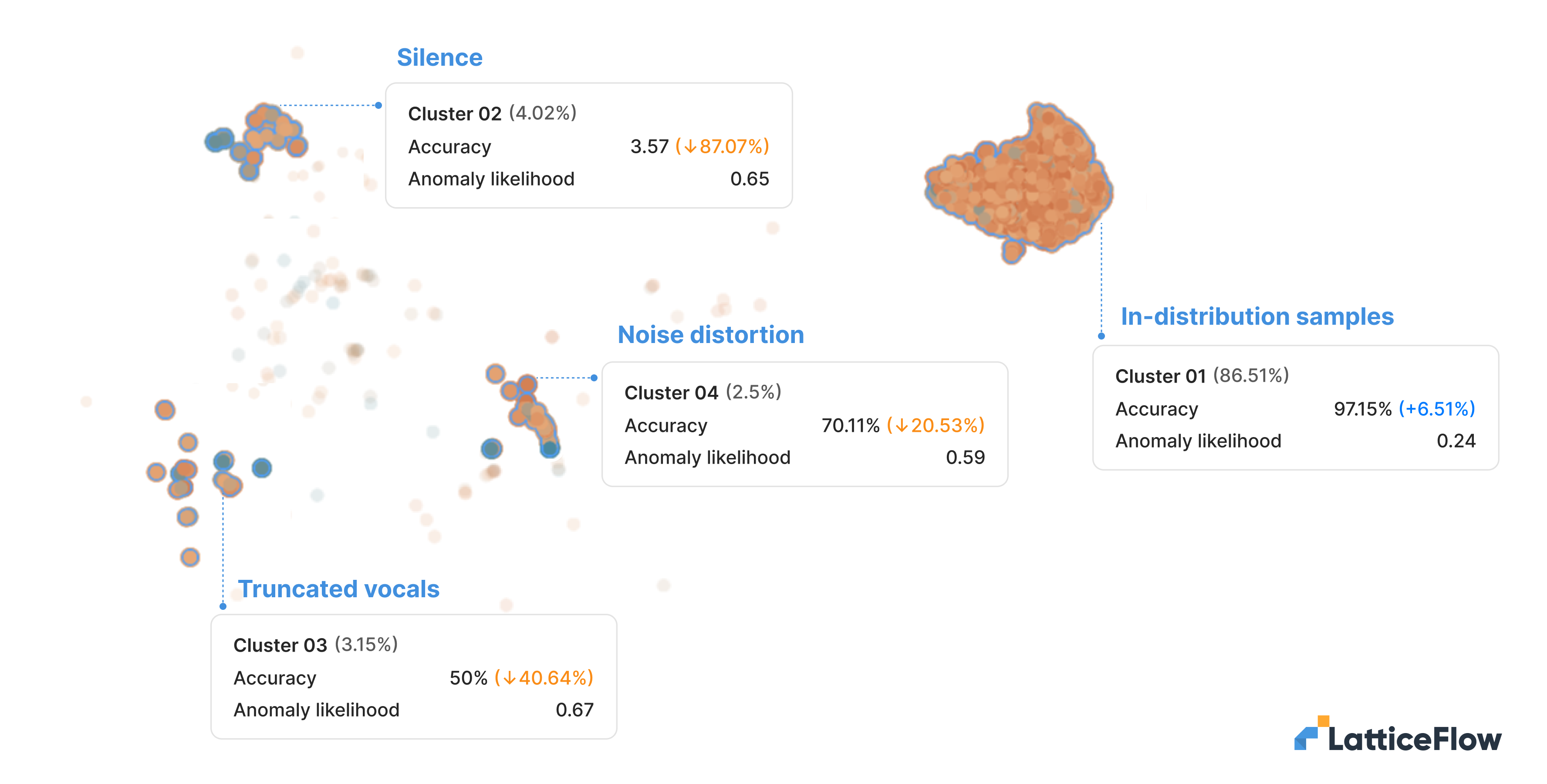
As we can see from the image below that shows embeddings for the command “house”, we can distinguish 4 clusters with unique characteristics:
- In distribution samples (Cluster 1): A cluster containing the majority of the data points for the filtered command, with an accuracy of 97,15%, performing better compared to the model’s overall performance. Most of the samples contained in this cluster are clearly spoken instances of the word by both male and female genders.
House (1) House (2) SpeechCommands: A DataSet for Limited-Vocabulary
- Silence (Cluster 2): A cluster consisting primarily of samples with the absence of speech with a substantial performance drop of 87.07% compared to overall performance.
House silence (1) House silence (2) SpeechCommands: A DataSet for Limited-Vocabulary
- Truncated vocals (Cluster 3): A cluster consisting of samples where the speech of the command is incomplete or cut off (e.g. only the first two letters are spoken). We can observe that the performance of these samples drops by 40% compared to overall performance when commands are fully spoken.
House truncated vocal (1) House truncated vocal (2) SpeechCommands: A DataSet for Limited-Vocabulary
- Noise distortion (Cluster 4): A cluster consisting mostly of samples where the speech is distorted by background noise. We can observe that background noise negatively affects the model performance by more than 20%.
House noise distortion (1) House noise distortion (2) SpeechCommands: A DataSet for Limited-Vocabulary

SpeechCommands: Embeddings clusters for the “speech” command word highlighting clusters of anomalies and the resulting degraded model performance.
After identifying individual cases of anomalous samples, the next step is to curate them by collecting all instances in the dataset based on their root cause and characteristics.
Curation of anomalies at scale
To curate anomalies at scale, we need a way to collect all samples based on their root cause or characteristics. As a concrete example, let’s try to find all occurrences of high-pitch recordings in the dataset. While one might attempt to reiterate the above procedure using embeddings, this approach doesn’t work in practice.
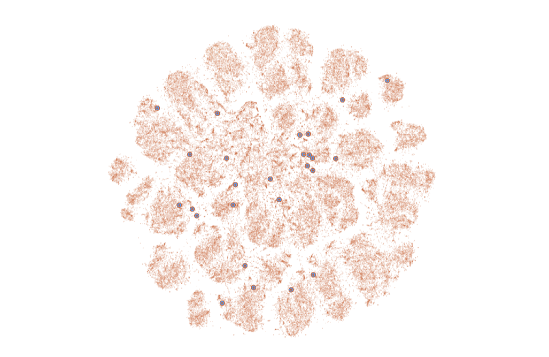
As we can see from the visualization below, where dataset data points are visualized using Embeddings and samples with high-pitched voices are highlighted, points of interest do not always cluster effectively. As a result, identifying high-pitched recordings using embeddings becomes very challenging, if not impossible.

Similarity search is an alternative method for retrieving samples similar to a given query. In our case, we could use anomalous samples as queries to identify all instances with high-pitch voices. Be aware that the effectiveness of the similary search is inherently limited by the explanatory power of the embeddings and is unlikely to perform effectively for this task.
Concepts are a new approach to automatically learn user-defined attributes and generalize them to unlabeled data through active learning. From the user perspective, the query can be the same as the one used for similarity search, but rather than simply using vector similarity in the embedding space, concepts learn their own featurerepresentation conditioned on the query. We can see the corresponding concept for high-pitch voice samples below.
SpeechCommands: A collection of all occurrences of high-pitch voices
After gathering all the samples, we can now determine the best course of action. While removing anomalies classified as silence is an intuitive action to take,the appropriate action for other scenarios depends on the use case. As a rule of thumb, scenario-based model monitoring is crucial for staying informed and keeping track of potential hidden degradation across model versions.
Conclusion
In this article, we analyzed the SpeechCommands dataset and identified several types of anomalous groups on the sample level (i.e. quality-specific anomalies, acoustic anomalies) as well as at the command level (i.e. truncated vocals, noise distortions, audio silence). Some of the anomalies correspond to hard samples for which the model does not generalize well and for which the next actionable step is to perform curation by targeted data collection and/or data augmentations. Other anomalies correspond to errors in the data preprocessing pipeline which significantly impact the accuracy of the model, highlighting the need to ensure that only high-quality data is included in the training.
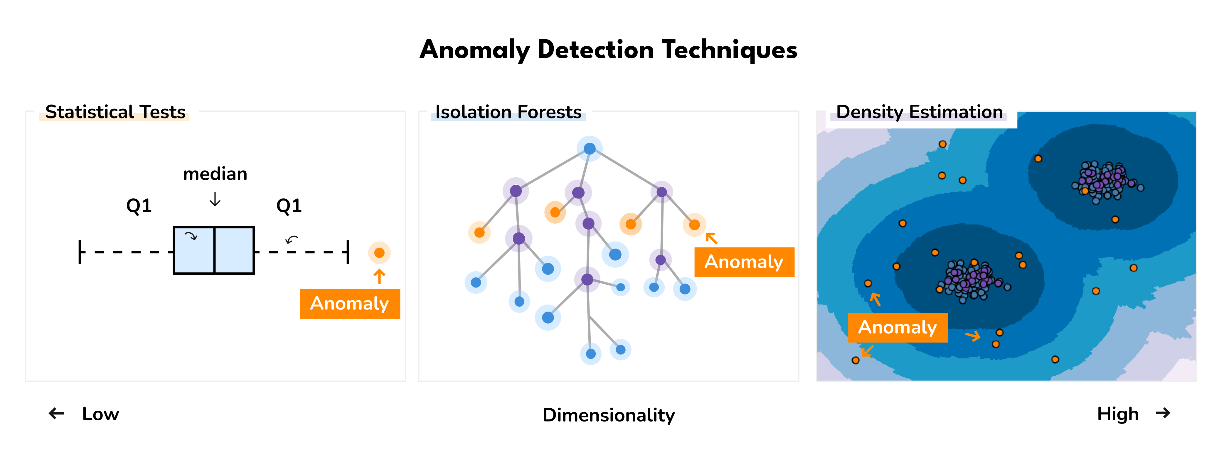
What was not covered in detail are the self-supervised techniques used to extract the correct feature representation as well as the concrete anomaly detection algorithms we used to detect them. For those interested in the details, existing research has been conducted to provide guidance on selecting the most appropriate algorithm, drawing from both theoretical perspectives [2] and benchmarks on real data. Emmott et al. (2015) found that isolation forest generally performs the best, but recommend using ABOG (Angle-Based Outlier Detection) or LOF (Local Outlier Factor) when the data contains multiple clusters.

For those interested in learning more, talk to our team at latticeflow.ai, where we focus on building intelligent workflows to help AI teams systematically identify and curate data and model issues at scale.
References:
- [1] Warden, P. (2018). Speech Commands: A Dataset for Limited-Vocabulary Speech Recognition. Google Research. https://doi.org/10.48550/arXiv.1804.03209
- [2] A. F. Emmott, S. Das, T. Dietterich, A. Fern, and W.-K. Wong. Systematic construction of anomaly detection benchmarks from real data. In Proceedings of the ACM SIGKDD workshop on outlier detection and description, pages 16–21, 2013.


